T. Pestana, M. Thalhammer, S. Hickel (2020)
Journal of the Atmospheric Sciences 77: 3193-3210. doi: 10.1175/JAS-D-19-0342.1
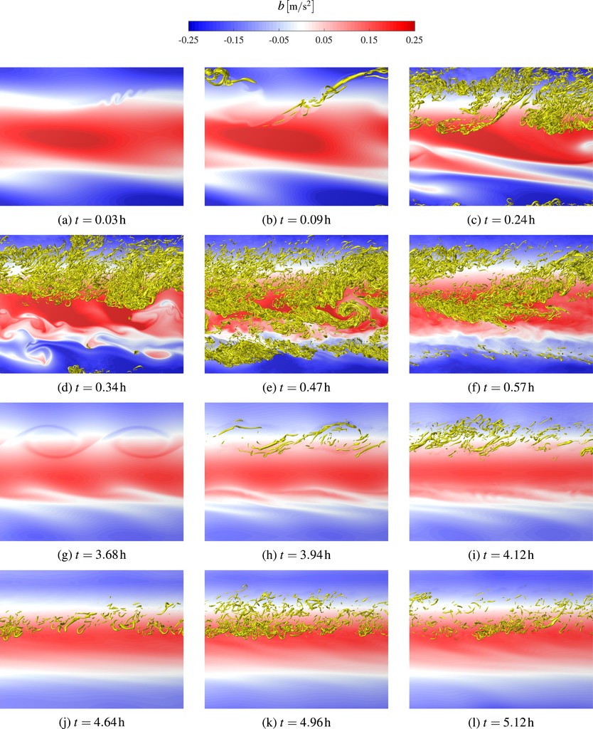
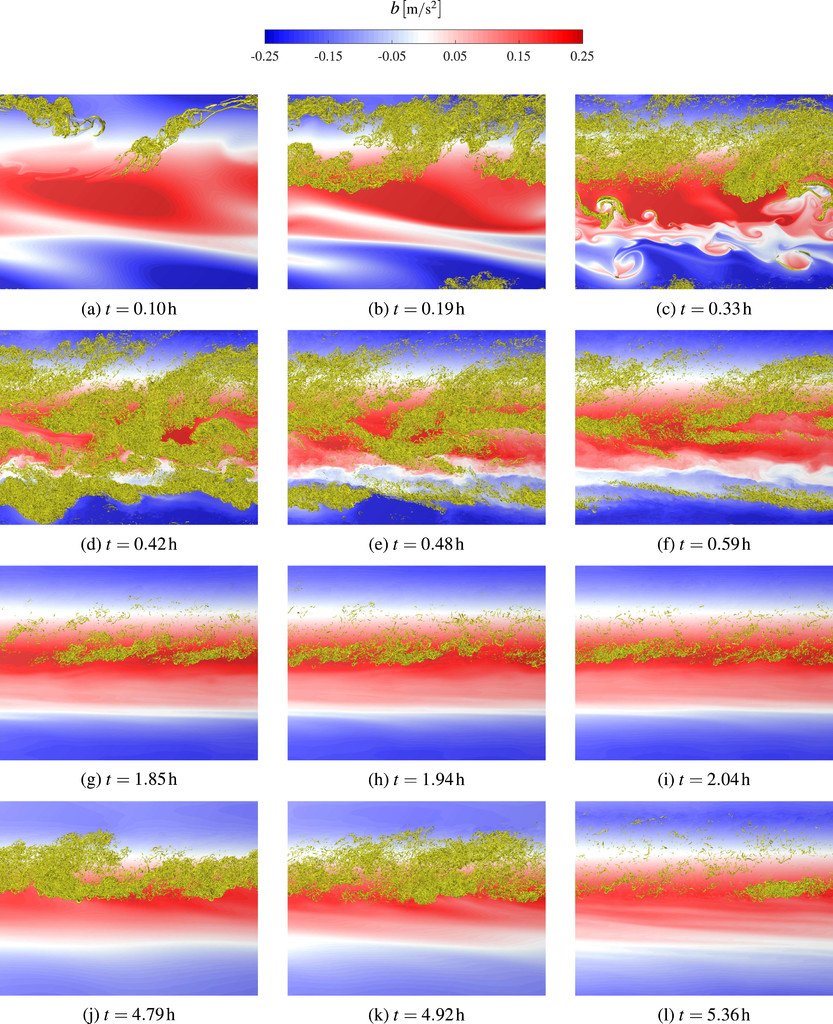
We present direct numerical simulations of inertia–gravity waves breaking in the middle–upper mesosphere. We consider two different altitudes, which correspond to the Reynolds number of 28 647 and 114 591 based on wavelength and buoyancy period. While the former was studied by Remmler et al., it is here repeated at a higher resolution and serves as a baseline for comparison with the high-Reynolds-number case.
The simulations are designed based on the study of Fruman et al., and are initialized by superimposing primary and secondary perturbations to the convectively unstable base wave. Transient growth leads to an almost instantaneous wave breaking and secondary bursts of turbulence. We show that this process is characterized by the formation of fine flow structures that are predominantly located in the vicinity of the wave’s least stable point.
During the wave breakdown, the energy dissipation rate tends to be an isotropic tensor, whereas it is strongly anisotropic in between the breaking events. We find that the vertical kinetic energy spectra exhibit a clear 5/3 scaling law at instants of intense energy dissipation rate and a cubic power law at calmer periods. The term-by-term energy budget reveals that the pressure term is the most important contributor to the global energy budget, as it couples the vertical and the horizontal kinetic energy. During the breaking events, the local energy transfer is predominantly from the mean to the fluctuating field and the kinetic energy production is in balance with the pseudo kinetic energy dissipation rate.